Tutorial: basic usage

This page walks you through the complete pyFracAggregate pipeline — generate, analyze, visualize, and export — twice: first a monodisperse aggregate built with particle-cluster aggregation (PCA), then a polydisperse aggregate built on the FracVAL coordinate. It is a static adaptation of the marimo notebooks, which remain in examples/ if you prefer an executable format — install with pip install -e ".[examples]" and run marimo edit examples/01_quickstart.py.

Every code block below was executed in the order shown, with pyFracAggregate 0.6.0 and seed=0 passed to each generation call. The printed values are the real measured outputs of that run, and the embedded figures are the actual artifacts of those exact calls (saved under different file names in the docs tree). If you run the snippets yourself you will get the same numbers; with a different seed you get a different realization, with a slightly different measured morphology.

Note

Plotting needs matplotlib, which is not installed by default: pip install "pyFracAggregate[plot]" (see Installation). 3D rendering uses pyvista, which is a base dependency.

Part 1 — monodisperse PCA aggregate

Generate the aggregate

Start with pfa.generate(), the single entry point for the whole coordinate system. We ask for 200 primary particles with a fractal dimension \(D_f = 1.8\) and prefactor \(k_f = 1.9\) — typical soot-like values (see Morphology parameters) — using method="pca", a fast particle-cluster baseline.

Pass seed= to generate(): generation is stochastic, and the seed is what makes a run reproducible (details in Reproducibility and seeding).

import pyFracAggregate as pfa

agg = pfa.generate(n_particles=200, df=1.8, kf=1.9, method="pca", seed=0)

print(f"Particles: {agg.current_size}")
print(f"Radii:     {agg.radii.min():.3f} to {agg.radii.max():.3f}")
extent = agg.positions.max(axis=0) - agg.positions.min(axis=0)
print(f"Extent:    {extent[0]:.1f} x {extent[1]:.1f} x {extent[2]:.1f} {agg.length_unit}")

Particles: 200
Radii:     1.000 to 1.000
Extent:    33.7 x 28.1 x 35.2 nm

With no particle_dist argument the primaries are monodisperse with radius 1.0 (in the default length_unit of nm), and 200 spheres at \(D_f = 1.8\) span roughly 35 nm — an open, branched object, not a compact ball.

Analyze morphology

pfa.analyze() computes the radius of gyration, center of mass, and — via the cumulative sandbox estimator — fractal-dimension estimates in both the counting and the mass measure, all in one call:

analyze() returns a typed MorphologyReport — read it by attribute:

report = pfa.analyze(agg)

print(f"Rg:        {report.rg:.3f} {agg.length_unit}")
print(f"CoM:       [{report.com[0]:.2f}, {report.com[1]:.2f}, {report.com[2]:.2f}]")
print(f"N:         {report.n}")
print(f"estimator: {report.estimator}")
print(f"Df,num:    {report.df_num_est:.3f}  (R2={report.r2_num:.4f})")
print(f"Df,mass:   {report.df_mass_est:.3f}  (R2={report.r2_mass:.4f})")

Rg:        13.274 nm
CoM:       [-3.62, 4.92, 0.15]
N:         200
estimator: sandbox
Df,num:    1.821  (R2=0.9798)
Df,mass:   1.821  (R2=0.9798)

For a monodisperse aggregate the mass measure is the counting measure times a constant, so df_mass_est equals df_num_est exactly — 1.821 twice above.

Read the last two lines with care. The estimated \(D_f\) is 1.821 against a request of 1.8 — close this time — and \(R^2 = 0.98\) says the log-log fit is good, but \(R^2\) measures fit quality, not agreement with the target. A single realization at moderate \(N\) typically deviates from the requested \(D_f\) by a few tenths (the pcf estimate below misses wider); average over several seeded realizations before quoting ensemble numbers (Interpreting df_num_est, df_mass_est and the r2 fields).

Pair correlation function

The pair correlation function is the classic differenced estimator of \(D_f\) from \(C(r) \propto r^{D_f - 3}\). Passing estimator="pcf" to pfa.analyze() walks this path instead of the sandbox — for this aggregate it reports df_num_est = 1.613 (r2_num = 0.9806), a wider miss from the 1.8 request than the sandbox’s 1.821 above. It is worth looking at the underlying curve: compute it explicitly, then let plot_pair_correlation() redraw it with the fractal fit and the fit window — the fit runs from the mean primary radius to \(R_g\):

r_centers, c_r = pfa.pair_correlation_function(agg, bins=50)
print(f"bins: {len(r_centers)}, r up to {r_centers[-1]:.1f} {agg.length_unit}")

pfa.plot_pair_correlation(
    agg,
    bins=50,
    show_fit=True,
    reference_df=1.8,
    save_path="pcf_pca.png",
)

bins: 50, r up to 38.3 nm
Plot saved to pcf_pca.png

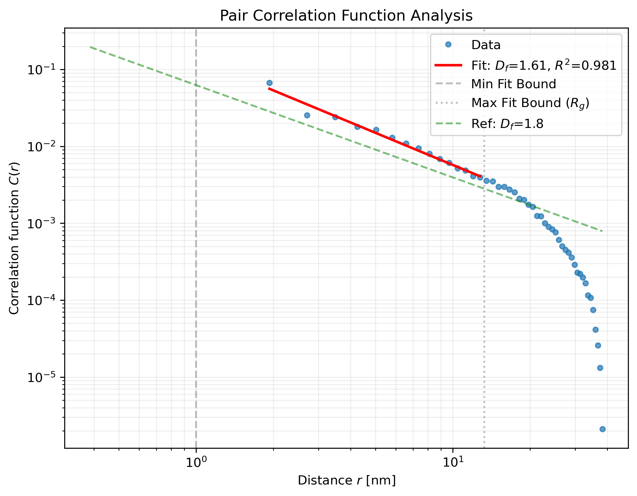
The pair correlation function of the 200-particle PCA aggregate. Blue dots: measured \(C(r)\). Red line: power-law fit over the fractal regime (slope \(= D_f - 3\)), giving \(D_f = 1.61\). Green dashed line: reference slope for the requested \(D_f = 1.8\). Vertical lines mark the fit window (mean primary radius to \(R_g\)).

The measured points follow a clean power law between the fit bounds and peel off at both ends — below the primary-particle scale and beyond \(R_g\), where finite-size effects dominate. That middle decade is exactly where the fractal dimension lives.

Render the aggregate

Numbers check out; now look at the object. save_screenshot() writes an off-screen 3D screenshot as PNG — window_size is capped at a modest 960 px to keep the docs light:

pfa.save_screenshot(agg, "pca_render.png", color="dimgray", window_size=(960, 720))

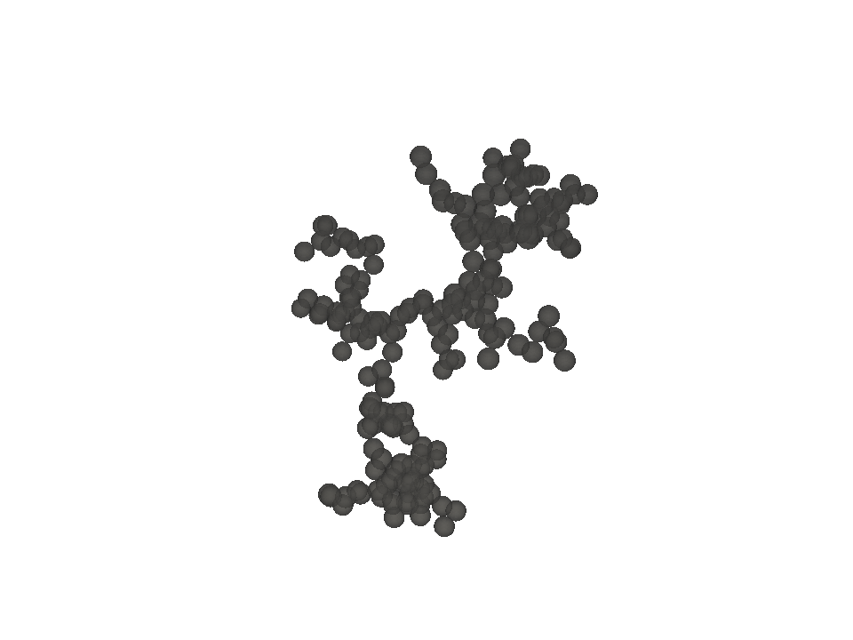
The 200-particle monodisperse PCA aggregate, rendered with pyvista. Every primary has radius 1.0 nm; the open, branched shape is the \(D_f = 1.8\) morphology.

Note

save_screenshot needs an OpenGL context even though it renders off-screen. On a headless server it may need xvfb-run or an OSMesa-built VTK — the workarounds are collected in Rendered image.

Export the data

Finally, persist the aggregate. export_yaml writes a full snapshot — particle data, units, and the generation parameters and analysis results you pass in (recording the seed makes the file traceable to an identical aggregate). export_yaml accepts the MorphologyReport directly and serializes it under the legacy snapshot key names. export_vtk writes a lightweight point cloud for ParaView:

pfa.export_yaml(
    agg,
    "aggregate.yaml",
    generation_params={"method": "pca", "n_particles": 200,
                       "df": 1.8, "kf": 1.9, "seed": 0},
    analysis_results=report,
)
pfa.export_vtk(agg, "aggregate.vtk")

This run produced a 23 KB aggregate.yaml and an 11 KB aggregate.vtk. Format guidance is in Exporting data — YAML for reproducibility, VTK point cloud for quick inspection, VTM MultiBlock when you need explicit sphere meshes.

Part 2 — polydisperse FracVAL-coordinate aggregate

Real soot primaries are not all the same size. Repeat the pipeline with a LognormalDistribution on the FracVAL coordinate — (method="cca", scaling="mass", placement="constructed") — which is designed for polydisperse primaries. Two things change in the call: the distribution and the coordinate — everything downstream (analyze, plotting, export) is identical.

poly = pfa.LognormalDistribution(mean=1.0, std=1.6)
agg_poly = pfa.generate(
    n_particles=256, df=1.8, kf=1.9,
    method="cca", scaling="mass", placement="constructed",
    particle_dist=poly, seed=0,
)

print(f"Particles:   {agg_poly.current_size}")
print(f"Radii:       {agg_poly.radii.min():.3f} to {agg_poly.radii.max():.3f}")
print(f"Mean radius: {agg_poly.radii.mean():.3f}")

Particles:   256
Radii:       0.232 to 4.225
Mean radius: 1.120

Two details worth noting:

• std is the geometric standard deviation. A value of 1.6 spreads the radii from 0.23 to 4.23 nm around a geometric mean of 1.0 nm — roughly a factor of eighteen between the smallest and largest primary. Values at or below 1.0 collapse to monodisperse (Particle size distributions).

• The coordinate accepts any particle count (\(N \leq 8\) internally falls back to a PCA call). 256 is simply a typical soot-aggregate size. (method="fracval" is a deprecated alias for exactly this coordinate.)

Analyze and compare

report_poly = pfa.analyze(agg_poly)

print(f"Rg:        {report_poly.rg:.3f} {agg_poly.length_unit}")
print(f"CoM:       [{report_poly.com[0]:.2f}, {report_poly.com[1]:.2f}, {report_poly.com[2]:.2f}]")
print(f"N:         {report_poly.n}")
print(f"Df,num:    {report_poly.df_num_est:.3f}  (R2={report_poly.r2_num:.4f})")
print(f"Df,mass:   {report_poly.df_mass_est:.3f}  (R2={report_poly.r2_mass:.4f})")

Rg:        17.068 nm
CoM:       [-9.22, -16.27, 0.73]
N:         256
Df,num:    1.782  (R2=0.9941)
Df,mass:   1.879  (R2=0.9763)

pfa.save_screenshot(agg_poly, "fracval_render.png", color="dimgray", window_size=(960, 720))

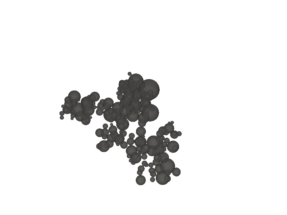
The 256-particle polydisperse aggregate on the FracVAL coordinate. Primary radii follow a lognormal distribution with geometric mean 1.0 nm and geometric standard deviation 1.6; the subcluster-merge construction gives a lumpier, more branched texture than the PCA aggregate of Part 1.

Sandbox measure comparison

pfa.plot_sandbox(
    agg_poly, show_fit=True, reference_df=1.8, measure="both",
    save_path="pcf_fracval_sandbox.png",
)

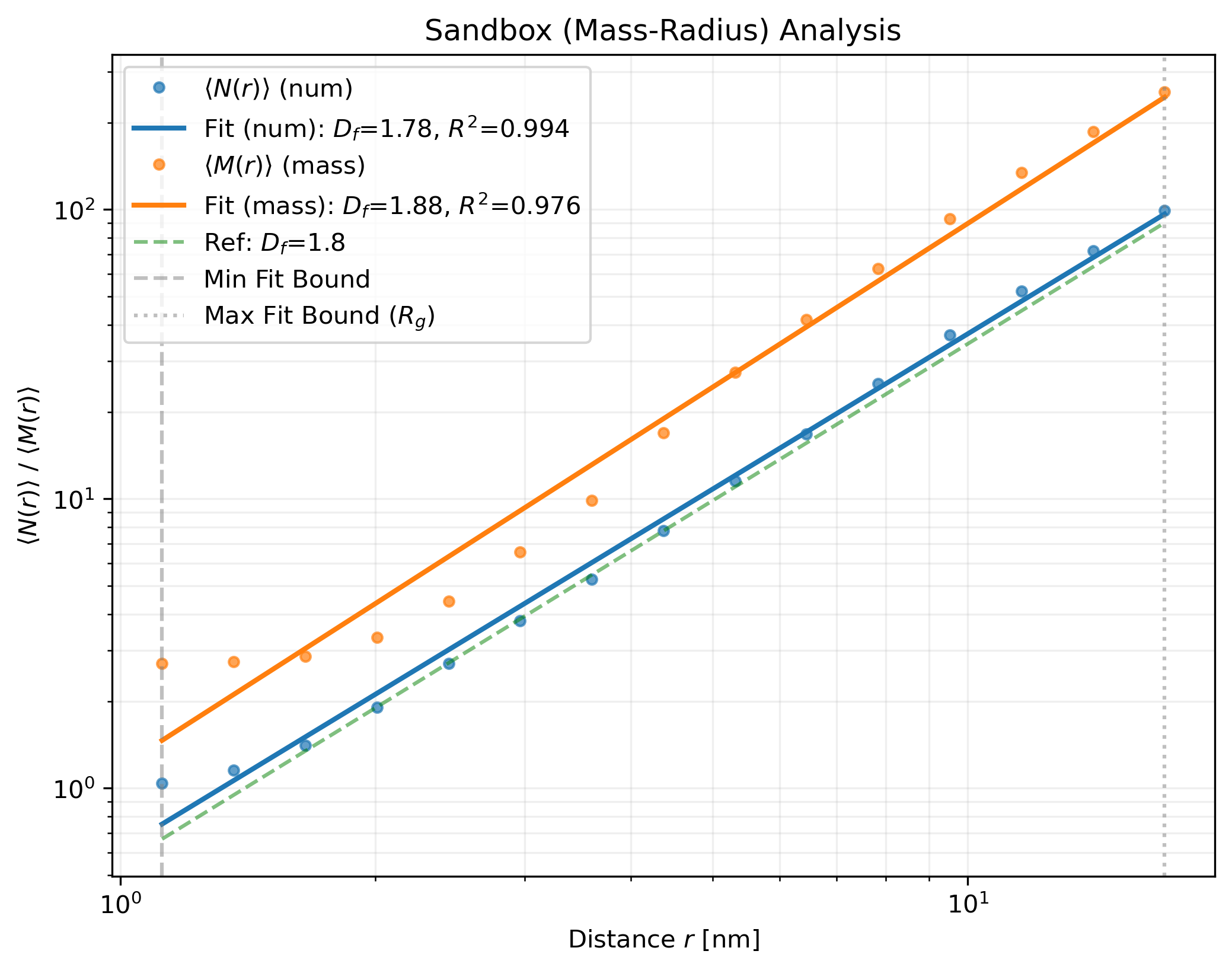
Both sandbox curves of the polydisperse aggregate. Blue: number measure ⟨N(r)⟩, fit \(D_{f,n}\) = 1.782. Orange: mass measure ⟨M(r)⟩ (≡ volume weighting at constant density), fit \(D_{f,m}\) = 1.879. Green dashed: reference slope for the requested \(D_f = 1.8\). The two exponents track the same arrangement here — radii are uncorrelated with position; see the background chapter.

Side by side, the two runs differ in three ways:

	Part 1 (PCA)	Part 2 (FracVAL coordinate)
Primaries	1.000 nm (monodisperse)	0.232–4.225 nm, lognormal
\(R_g\)	13.274 nm	17.068 nm
df_num_est (\(R^2\))	1.821 (0.9798)	1.782 (0.9941)
df_mass_est (\(R^2\))	1.821 (0.9798)	1.879 (0.9763)

• Polydispersity. The radius spread is the whole point of Part 2: large primaries anchor the cluster while small ones fill the crevices, which is what real combustion soot looks like (Primary particles).

• Construction. PCA accretes one particle at a time onto a growing cluster; the FracVAL coordinate grows small subclusters first and merges them cluster-to-cluster, so the render shows a lumpier, more branched object (The coordinate system).

• Size and Df. With the same \(D_f\) and \(k_f\) requested (and a somewhat larger \(N\)), the FracVAL cluster has a larger \(R_g\) (17.1 vs 13.3 nm) — the scaling-law targets are statistical, not exact per realization. This realization’s sandbox estimates straddle the 1.8 request (df_num_est = 1.782 just under, df_mass_est = 1.879 above), while Part 1’s two values coincide at 1.821 — with monodisperse primaries the mass measure is the counting measure times a constant, so the equality is exact, not a coincidence. Same lesson either way: one realization is one sample; seed several and average when you report morphology.

Where to go next

• Generating aggregates — all generate() parameters, the scaling axis, placement strategies, seeding.

• Analyzing aggregates — the individual analysis functions and choosing the fit window.

• Exporting data — the five export formats, ParaView workflows, headless-rendering workarounds.

• Background — what \(D_f\) and \(k_f\) mean and how each algorithm approximates them.

• API reference — full signatures.